SECTIONS
Introduction | Gambling & Probabilities | Shaping the Risk/Reward ProfileSo should we play Black Jack instead? | Insurance | Investing | Conclusions
This is part 2 of a 4-part article that begins here.
Shaping the Risk/Reward Profile
In the previous section I wrote about expected results, but that's only part of the story. We know that our expected result at the roulette is to lose 1/18 of all we bet, but we may want to know what chances we have of winning something. These kinds of questions require a more detailed description of the possible outcomes of the game, one that can be provided by a graph. I'm going to explain a very basic kind of graph used in probability theory, called a probability density graph. If you have Probability 101 covered, then this part will probably bore you. If you haven't, you might pick a few ideas that can become useful for investing.
We explained before that betting on a color at the roulette gave you an 18-in-38 chance of winning, and thus a 20-in-38 chance of losing. Let's say we bet $16 on a color, and graph the possible results:
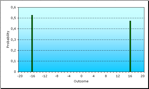
The x-axis shows possible outcomes and the y-axis its probabilities. This is called a probability density graph. After the spin we will either have won $16 or have lost $16, so all other outcomes are shown with zero probability, while the possible ones have approximately half a chance each. The probability to lose is a bit higher, because it is 20/38 against 18/38.
What if, instead of putting $16 in a single bet, we bet at two spins, $8 each time? The following is the probability density of this other play:
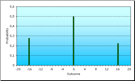
As can be seen, the outcomes are now three: we can either win twice, lose twice, or win one and lose the other, breaking even. The higher probability is allocated to the case of breaking even. The chances of losing $16 are now slimmer, so betting like this would be a more conservative move, to make our money last longer. Nevertheless, observe that the chances of winning are also much lower. Not just that, if we compare the probability of winning something (in this case, $16) to that of losing, the relation is also lower. Before, the chances of winning $16 were equal to a 90% of the chances of losing them, but now they are only a 81%. Lets see what happens with the graph if we bet one dollar 16 times:
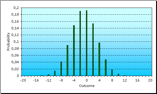
An interesting bell shape is starting to appear. The probability density is actually tending to the well-known Normal Bell Curve, also known as Gauss Bell, because that is what happens when unrelated probability densities are accumulated (and this is why the Gauss Bell is so important). What we see are samples of a symmetric Gauss Bell, where the samples are taken at the possible outcomes. If we average all outcomes, weighting them according to their probability, we will obtain the value, on the outcome axis, that is crossed by the line of symmetry of the bell. Can you deduce which number this is? It is the expected result of your game at the roulette, which, as we said in the previous part, is equal to 1/18 of the $16 that we bet, or 89 cents.
The previous graphs have the same expected value, because the total bet is the same. The difference resides in the shapes of the graphs. The first one has a very sparse, open shape, with high values at the extremes and nothing in the middle. The chances of losing $16 are quite high there. As we distribute the $16 among more spins, the probability concentrates at the middle (this is, the minus 89 cents). This effect is called the Law of Large Numbers, which I had mentioned previously. When we observed that the probability of winning became smaller compared to that of losing, it was a corollary of the concentration of probability around the expected value, which is on the losing side.
As we distribute the money among more spins, the probability concentrates at the middle
As a side note, let me mention that the "sparseness" or "un-concentration around the expected value" of these kinds of graphs can be described by a measure called standard deviation, which is frequently used in Modern Portfolio Theory. When we distribute the bets among unrelated spins, or should I say "diversify the bet", the standard deviation decreases, or put in investing terms, the risk diminishes. This is one way of shaping the risk/benefit to our desires, which may be wise if our intention is to last more at the table, but done excessively for this case makes no sense... Why would we want to obtain a predictable result around minus 89 cents?
Do you see the importance of casino profits in this argument? With expected values being negative, it is useless to diminish risk as much as we can, because we would only be ensuring a negative result. That isn't the case with investing. We will return to that shortly.
 Subscribe